Three ways to implement recursive circuits in the Faust language
After a long silence, this post is about the implementation of not-so-simple recursive circuits in the Faust language. We will see a few relevant examples and the three main approaches that we can follow to implement a circuit: Faust’s diagram expressions (basic syntaxt), the with environment with auxiliary function definition, and the letrec environment.
The Faust manual provides basic examples for the first, second, and third approaches. As we will see later, Faust’s basic syntax can be less concise and more complicated in some cases, whereas the remaining two approaches are easier. However, the letrec environment, despite being concise, is not always desirable if we want to generate diagrams that have little or no redundancy. In this post, we will implement a few circuits with feedback using all of the three approaches.
Let’s start with a simple one-pole lowpass filter, which is essentially a scaled-down input feeding into an integrator. In the basic syntax, the tilde operator lets the signal(s) to its left through and sendsthem back into a feedback path to fill the first available input(s) in the function. The operand or group of operands immediately after the tilde operator is applied to the feedback path. The tilde operator, unlike all other basic synthax operators, is left-assiociative and has highest priority. For example, if we write:
1
2
import("stdfaust.lib");
process = + , _ : + : + ~ _;
we are summing the first two inputs, then we are sending the result together with a third input into another “+” operator, and then we are summing the result to the output itself. Of course, any feedback loop in a digital system requires at least a one-sample delay, which is the default delay in Faust’s recursive composition. Suppose that we want to add another feedback loop in the previous function that is connected to the input of the first “+” operator. We also want to multiply that feedback signal by .5. Then we can write as follows:
1
2
import("stdfaust.lib");
process = (+ , _ : + : + ~ _) ~ *(.5);
Back to the lowpass filter, we can see the diagram below, kindly taken from the website of Julius Smith.
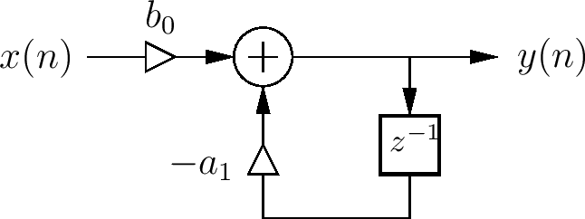
Following [Chamberlin 1985] for the design of the filter, we can write the function using basic syntax as follows:
1
2
3
4
5
6
7
8
import("stdfaust.lib");
lowpass(cf, x) = b0 * x : + ~ *(-a1)
    with {
        b0 = 1 + a1;
        a1 = exp(-w(cf)) * -1;
        w(f) = 2 * ma.PI * f / ma.SR;
    };
process = lowpass;
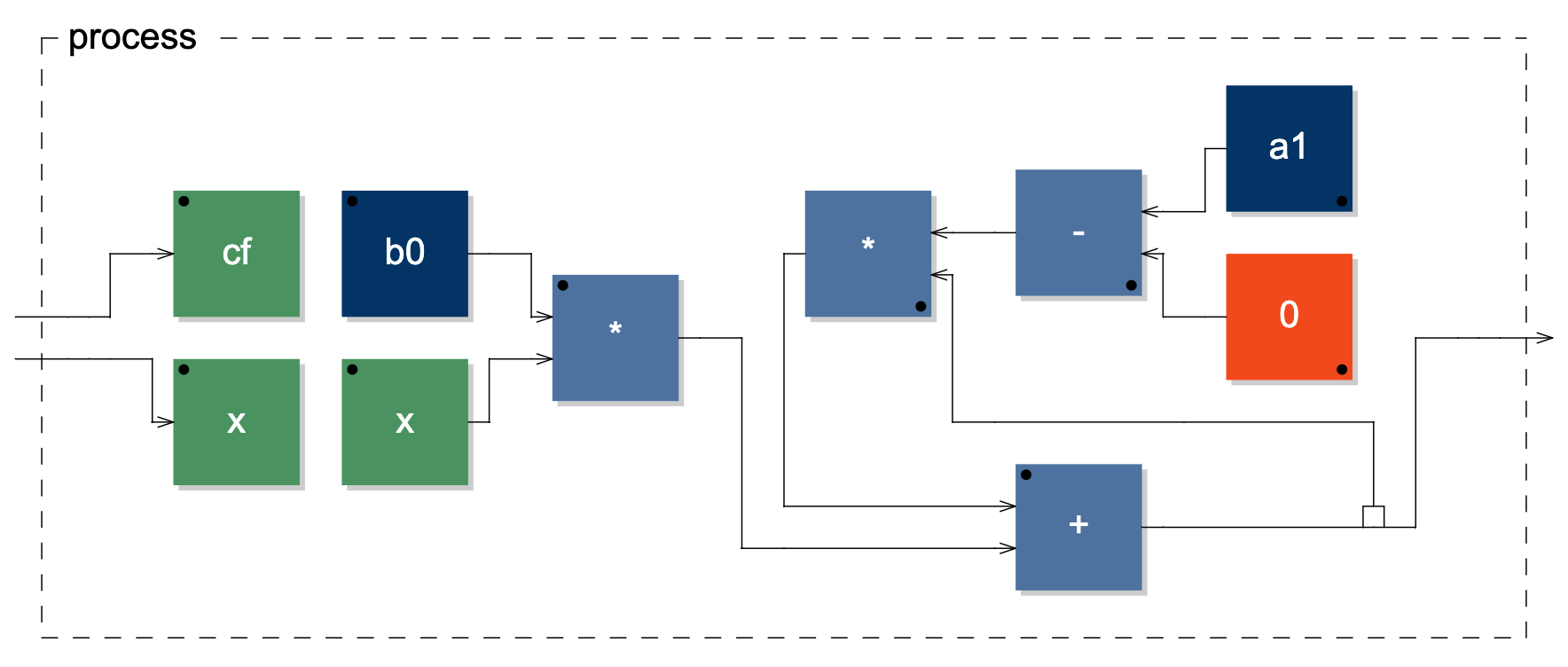
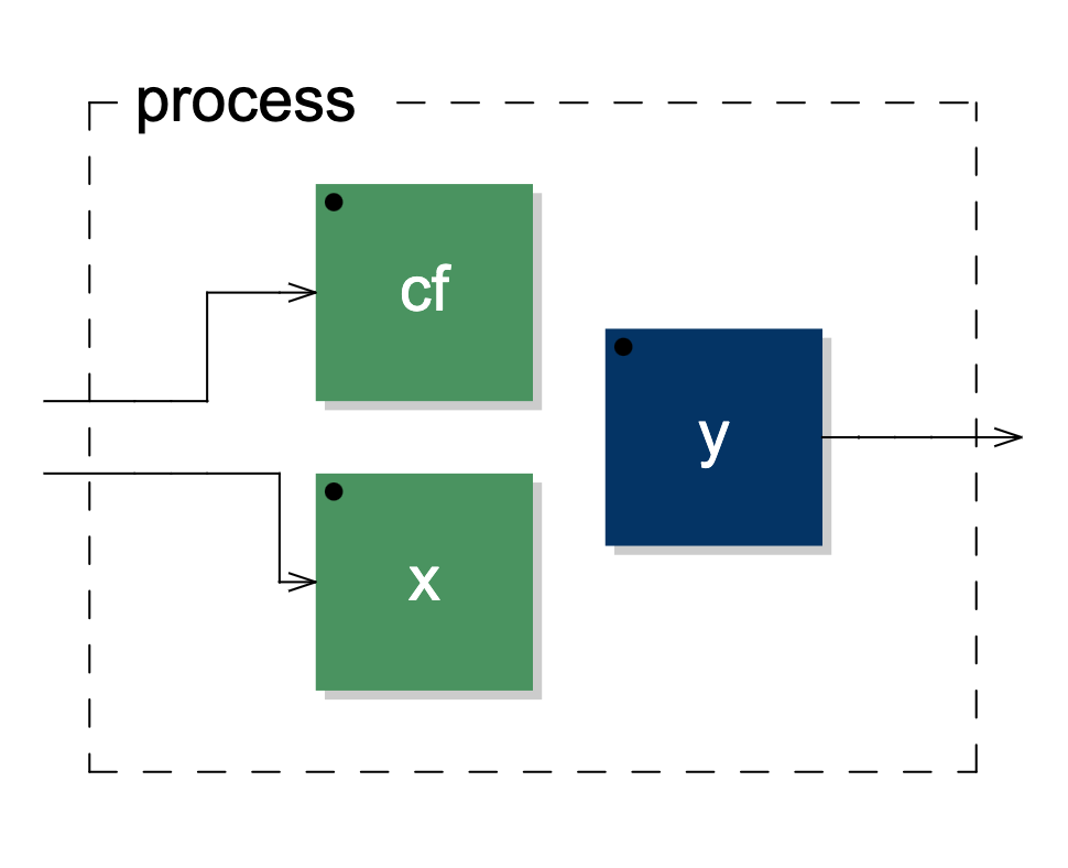
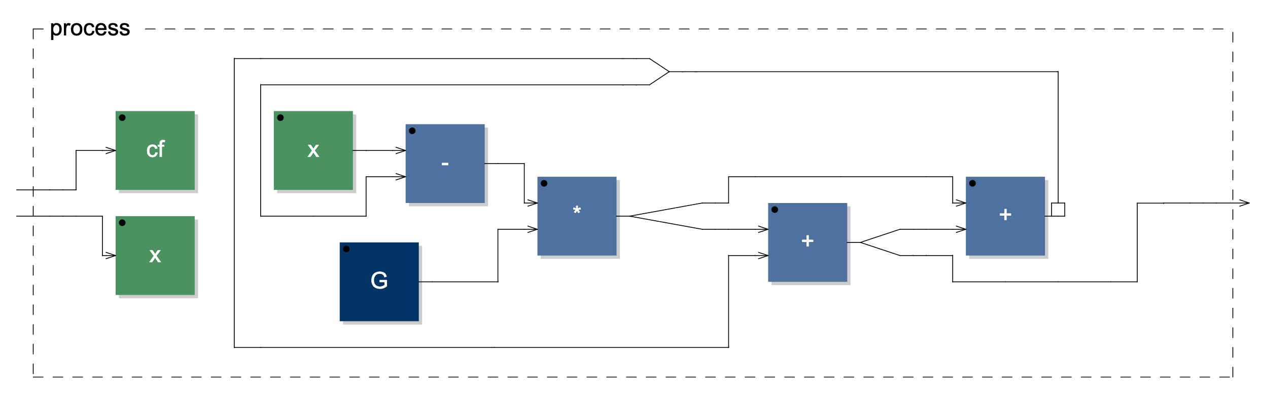
Below, we can see the diagram generated by the Faust code. Note that the empty little square on a wire indicates a one-sample delay, representing the $ z^-1 $ operator in our case.
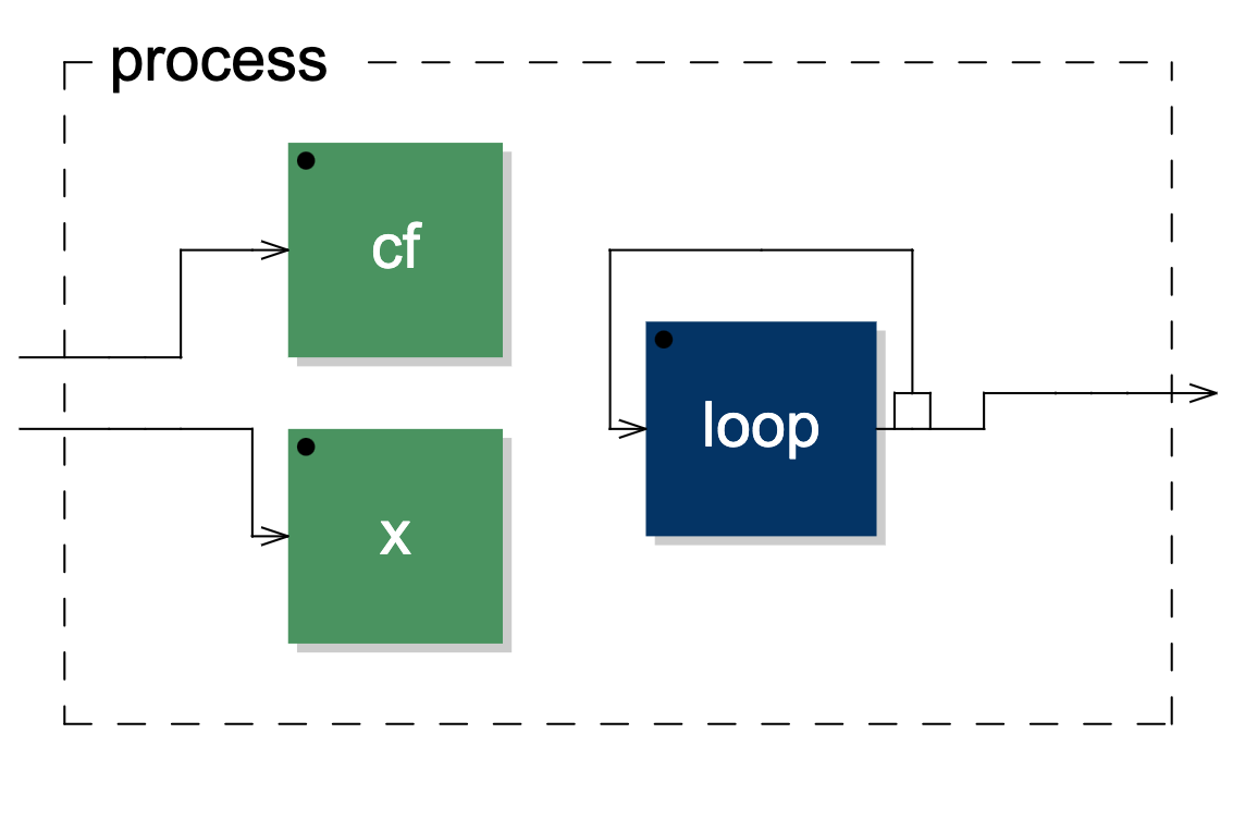
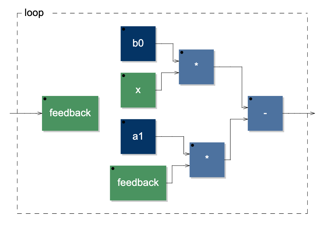
Another way to implement the filter is by using an intermediate function and the with environment. I would also like to thank Oleg Nesterov who first introduced me to this technique. The intermediate function usually acts as container and defines elementary single or multiple feedback loops. The feedback loops that are sent back to the function can then be used anywhere in the inner code as they are identified by argument names, which are specified in the intermediate function (“loop”) definition:
1
2
3
4
5
6
7
8
9
import("stdfaust.lib");
lowpass(cf, x) = loop ~ _
    with {
        loop(feedback) = b0 * x - a1 * feedback;
        b0 = 1 + a1;
        a1 = exp(-w(cf)) * -1;
        w(f) = 2 * ma.PI * f / ma.SR;
    };
process = lowpass;
The third way is through the letrec environment. Within this environment, we can define signals recursively, similarly to how recurrence equations are written:
1
2
3
4
5
6
7
8
9
10
11
import("stdfaust.lib");
lowpass(cf, x) = y
    letrec {
        'y = b0 * x - a1 * y;
    }
        with {
            b0 = 1 + a1;
            a1 = exp(-w(cf)) * -1;
            w(f) = 2 * ma.PI * f / ma.SR;
        };
process = lowpass;
So far, we have implemented a somewhat elementary circuit. Now, we can try to implement a first-order lowpass filter with zero-delay feedback topology. The circuit below is taken from the book by Zavalishin on virtual analogue filters design.
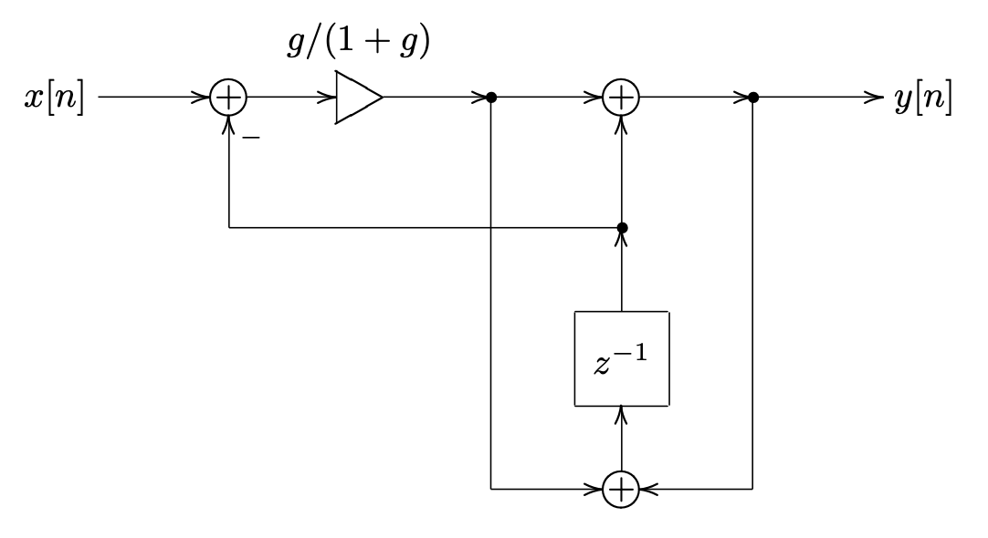
As we can see, the implementation is not as straightforward as the previous case. It can be useful to name several points in the circuit to determine the fundamental signals to compose the whole circuit. Here, we introduce $ G = g/(1+g) $, $ v $ as the signal taken after the $ G $ multiplication, $ s $ as the state of the system, that is the output of the $ z^-1 $ operator, and $ y $ as the output of the system. Hence, we have that:
\[\begin{align} & v = G(x - s) \\ & y = v + s \\ & s = v + y \\ \end{align}\]If we substitute $ v $ and $ y $, then we have that:
\[\begin{align} & y = G(x - s) + s \\ & s = 2G(x - s) + s \\ \end{align}\]and we can define two paths, one for the state, the other for the output of the system. Specifically, we can write the paths replacing all occurrences of $ s $ with a wire, which we will then fill with feedback loops from the state path. It is convenient to define the state first, and the output second, as the tilde operator applies to signals to its left starting from the top:
1
2
3
4
5
6
7
8
9
import("stdfaust.lib");
lowpass(cf, x) =
    (2 * (x - _) * G + _ , // state path
    (x - _) * G + _) ~ (_ <: si.bus(4)) : ! , _ // output path
    with {
        G = tan(w(cf) / 2) / (1 + tan(w(cf) / 2));
        w(f) = 2 * ma.PI * f / ma.SR;
    };
process = lowpass;
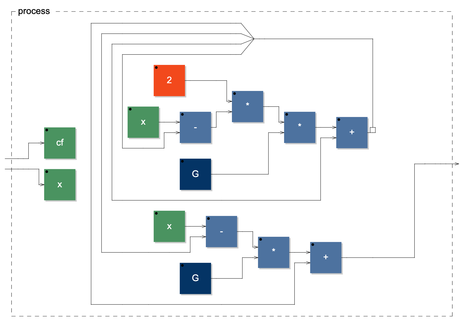
As we can notice, the signal $ G(x - s) + s $ repeats twice in the diagram. However, Faust’s optimisation will make sure that the signal is computed only once. Still, if we want the diagram to be closer to the original circuit, then we can write the following, copying the signal $ G(x - s) $ internally to compose the remaining necessary signals:
1
2
3
4
5
6
7
8
import("stdfaust.lib");
lowpass(cf, x) =
    (((x - _) * G <: _ , _) , _ : (_ , (+ <: _ , _)) : (+ , _)) ~ (_ <: si.bus(2)) : ! , _
    with {
        G = tan(w(cf) / 2) / (1 + tan(w(cf) / 2));
        w(f) = 2 * ma.PI * f / ma.SR;
    };
process = lowpass;
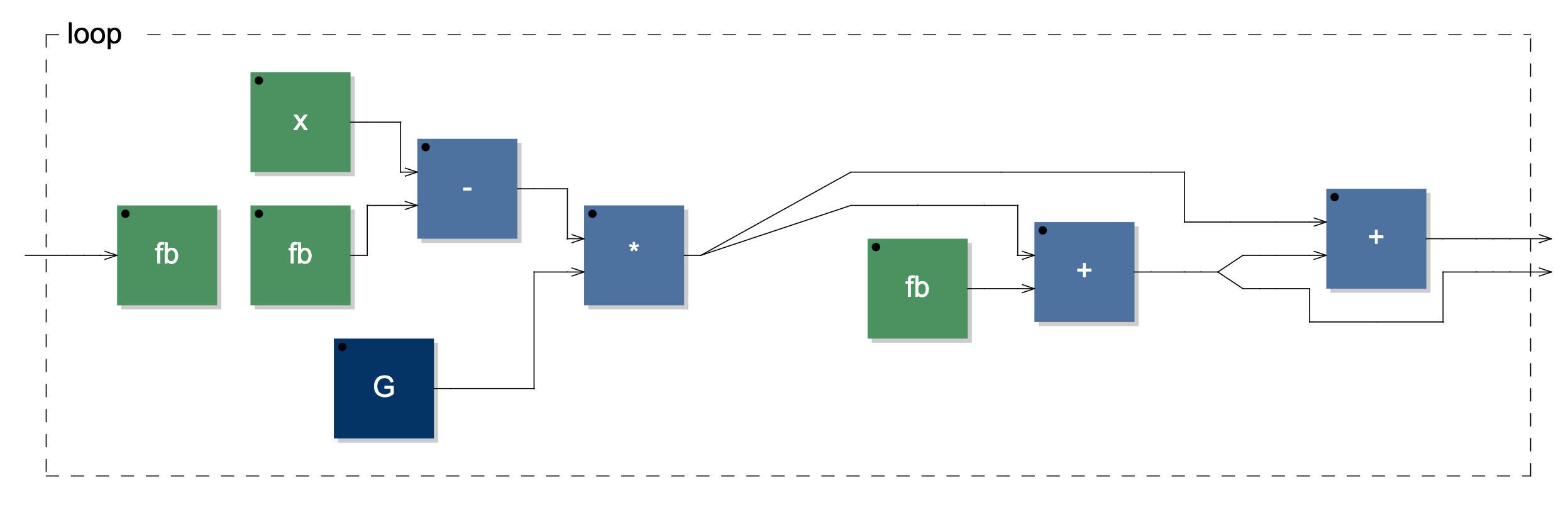
Now, we can implement the filter using an intermediate function:
1
2
3
4
5
6
7
8
import("stdfaust.lib");
lowpass(cf, x) = loop ~ _ : ! , _
    with {
        loop(fb) = (x - fb) * G <: _ , +(fb) : _ , (_ <: _ , _) : + , _;
        G = tan(w(cf) / 2) / (1 + tan(w(cf) / 2));
        w(f) = 2 * ma.PI * f / ma.SR;
    };
process = lowpass;
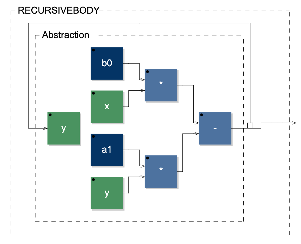
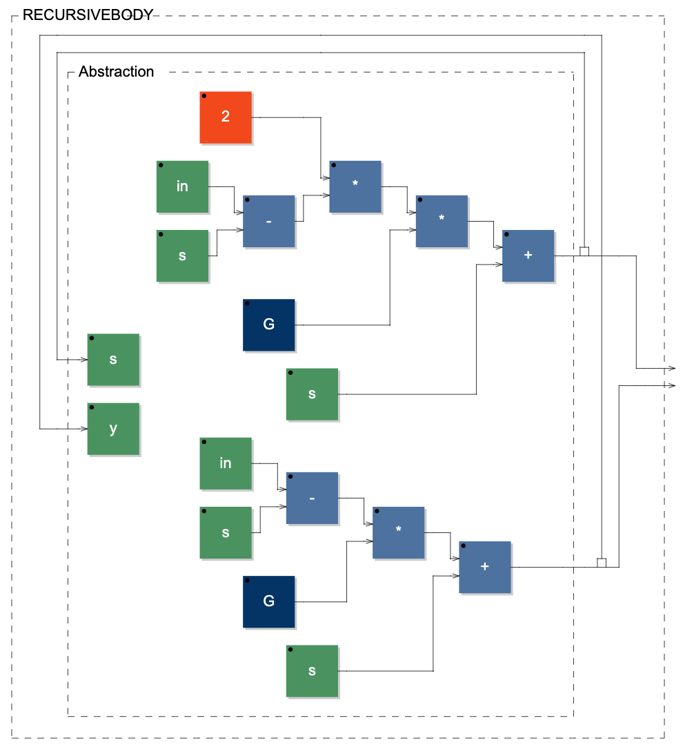
And finally, we can use the letrec environment for a concise and elegant solution, although the diagram will show some redundancy:
1
2
3
4
5
6
7
8
9
10
11
import("stdfaust.lib");
lowpass(cf, in) = y
    letrec {
        'y = (in - s) * G + s;
        's = 2 * (in - s) * G + s;
    }
        with {
            G = tan(w(cf) / 2) / (1 + tan(w(cf) / 2));
            w(f) = 2 * ma.PI * f / ma.SR;
        };
process = lowpass;
For the last example, we will implement Martin Vicanek’s beautiful quadrature oscillator, a recursive self-oscillating system with two states. See the circuit below.
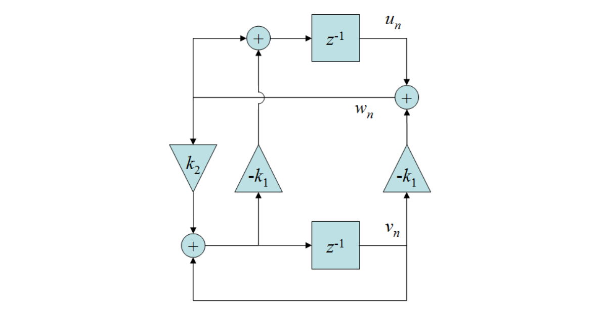
Here, we have a feedback system with two cross-coupled states. Hence, it is not as straightforward as with systems having only one state, for we must send each state back to the appropriate inputs. In this system, we need to define two state paths, which correspond to the two outputs of the system. Similarly to what we did earlier, we can define the states by composing the paths with the signals feeding into the $ z^-1 $ operators. Thus, the two states $ u_n $ and $ v_n $ are defined as follows:
\[\begin{align} & u_n = w_n - k_1(v_n + k_2 \cdot w_n) \\ & v_n = v_n + k_2 \cdot w_n \\ & w_n = u_n - k_1 \cdot v_n \\ \end{align}\]If we substitute $ w_n $, we have that:
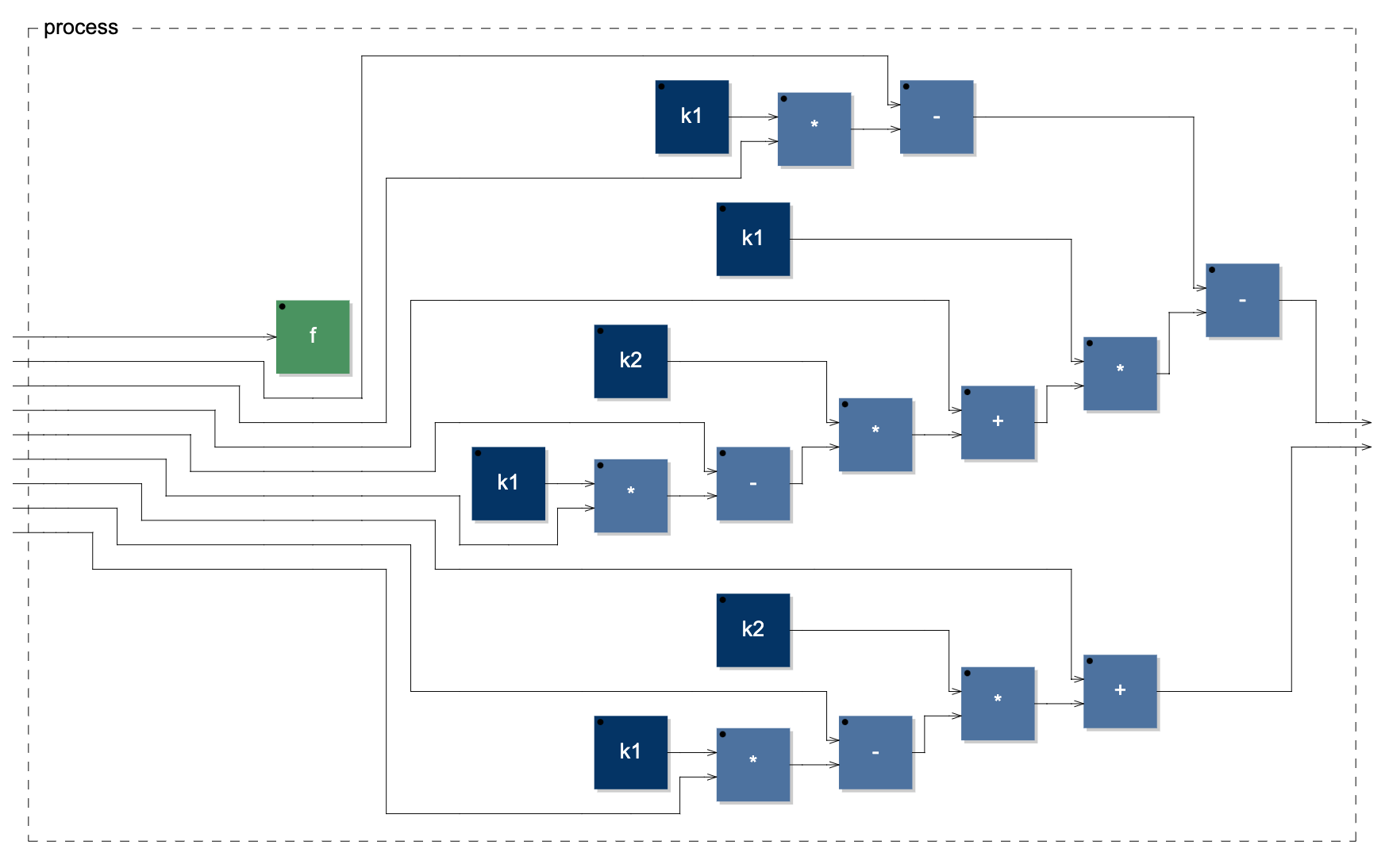
\[\begin{align} & u_n = u_n - k_1 \cdot v_n - k_1(v_n + k_2(u_n - k_1 \cdot v_n)) \\ & v_n = v_n + k_2(u_n - k_1 \cdot v_n) \\ \end{align}\]To start with, using basic syntax, we will simply put a wire wherever a state is fed back without distinguishing between $ u_n $ or $ v_n $:
1
2
3
4
5
6
7
8
import("stdfaust.lib");
quadosc(f) =    (_ - k1 * _ - k1 * (_ + k2 * (_ - k1 * _)) ,    // u_n path
                _ + k2 * (_ - k1 * _))                          // v_n path
    with {
        k1 = tan(ma.PI * f / ma.SR);
        k2 = (2 * k1) / (1 + k1 * k1);
    };
process = quadosc;
This will lead to the following network, where the external inputs are feedback paths that need to be matched with the corresponding states.
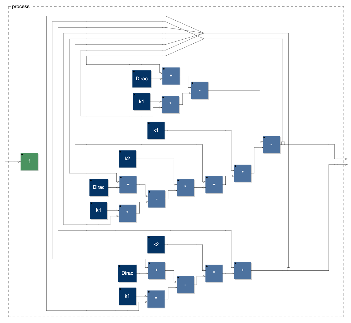
At this point, and without worrying about redundancy in the resulting diagram, the easiest thing to do is to send the two states to the feedback path and then copy and route them accordingly. We can do so using the “route” primitive, which we can call specifying the number of inputs, the number of outputs, and a set of input-output pairs to route the signals. Furthermore, we will also add a one-sample impulse to the $ u_n $ state as its initial condition must be 1.
1
2
3
4
5
6
7
8
9
10
11
import("stdfaust.lib");
quadosc(f) =
    (_ + Dirac - k1 * _ - k1 * (_ + k2 * (_ + Dirac - k1 * _)) ,    // u_n path
    _ + k2 * (_ + Dirac - k1 * _))                                  // v_n path
    ~ route(2, 8, 1, 1, 2, 2, 2, 3, 1, 4, 2, 5, 2, 6, 1, 7, 2, 8)
    with {
        k1 = tan(ma.PI * f / ma.SR);
        k2 = (2 * k1) / (1 + k1 * k1);
        Dirac = 1 - 1';
    };
process = quadosc;
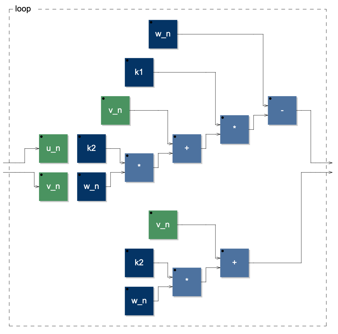
Next, we can see how to implement the oscillator using the second approach. It should be clear now:
1
2
3
4
5
6
7
8
9
10
11
12
13
import("stdfaust.lib");
quadosc(f) = loop ~ (_ , _)
    with {
        loop(u_n, v_n) =    w_n - k1 * (v_n + k2 * w_n) ,   // u_n path
                            v_n + k2 * w_n                  // v_n path
            with {
                w_n = Dirac + u_n - k1 * v_n;
            };
        k1 = tan(ma.PI * f / ma.SR);
        k2 = (2 * k1) / (1 + k1 * k1);
        Dirac = 1 - 1';
    };
process = quadosc;
Lastly, we can see how to implement the system using letrec:
1
2
3
4
5
6
7
8
9
10
11
12
import("stdfaust.lib");
quadosc(f) = u_n , v_n
    letrec {
        'u_n = Dirac + u_n - k1 * v_n - k1 * (v_n + k2 * (Dirac + u_n - k1 * v_n));
        'v_n = v_n + k2 * (Dirac + u_n - k1 * v_n);
    }
        with {
            k1 = tan(ma.PI * f / ma.SR);
            k2 = (2 * k1) / (1 + k1 * k1);
            Dirac = 1 - 1';
        };
process = quadosc;
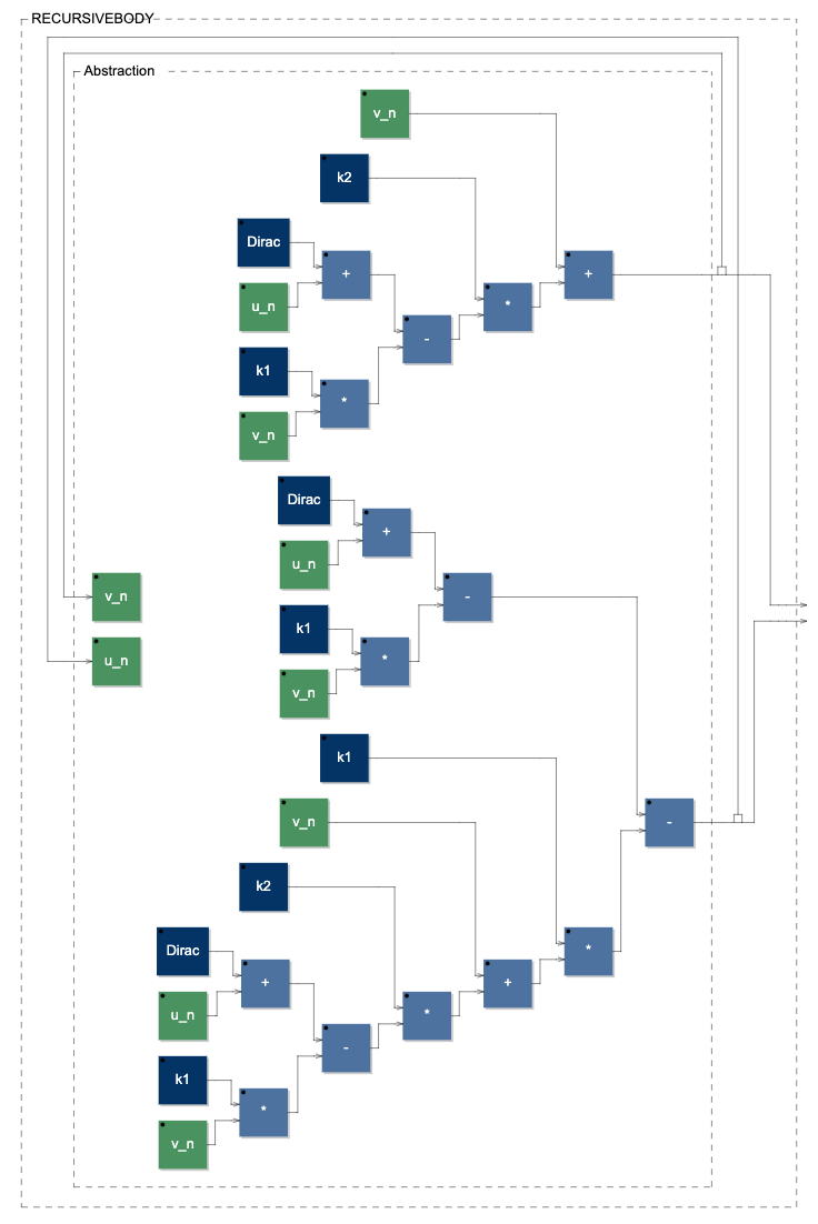
Overall, it seems that the with and letrec environments are best to work with. Particularly the with environment with auixiliary function, it allows to define temporary or intermediate signals as we did for the quadrature oscillator. Using letrec, instead, that would not be possible as it would introduce a delay in the auxiliary path. The basic syntax, though, is still useful when we want to generate diagrams showing the entire network topology.