Efficient exponential interpolation using one-pole filters
Exponential curves are particularly useful in digital audio as they provide natural-sounding amplitude variations, and they describe the behaviour of dis/charging capacitors in analogue RC circuits [Chamberlin 1985]. A common task, among others, is modelling analogue ADSR envelope generators, which are based on such circuits.
Digital one-pole filters can emulate these circuits, although they would require infinite time to reach the target value exactly. Nigel Redmon from Earlevel Engineering has addressed this problem using overshooting one-pole filters, which he discusses in a series of blog posts. Here, we will see a solution following the same principle but with a slightly different formalisation that turns one-pole filters into an exponential mapping function with arbitrary dis/charging rates passing through two arbitrary values. This is useful as it allows computing the exponential interpolation using one multiply and two sums per sample rather than one exponential function and one multiply.
Given start and end values, respectively, $ y_0 $ and $ y_1 $, there is an infinite family of exponential mapping functions connecting these two points:
$$ \begin{equation} f(x) = \frac{1-e^{-kx}}{1-e^{-k}}(y_1 - y_0) + y_0 \tag{1} \label{eq:expInter} \end{equation} $$
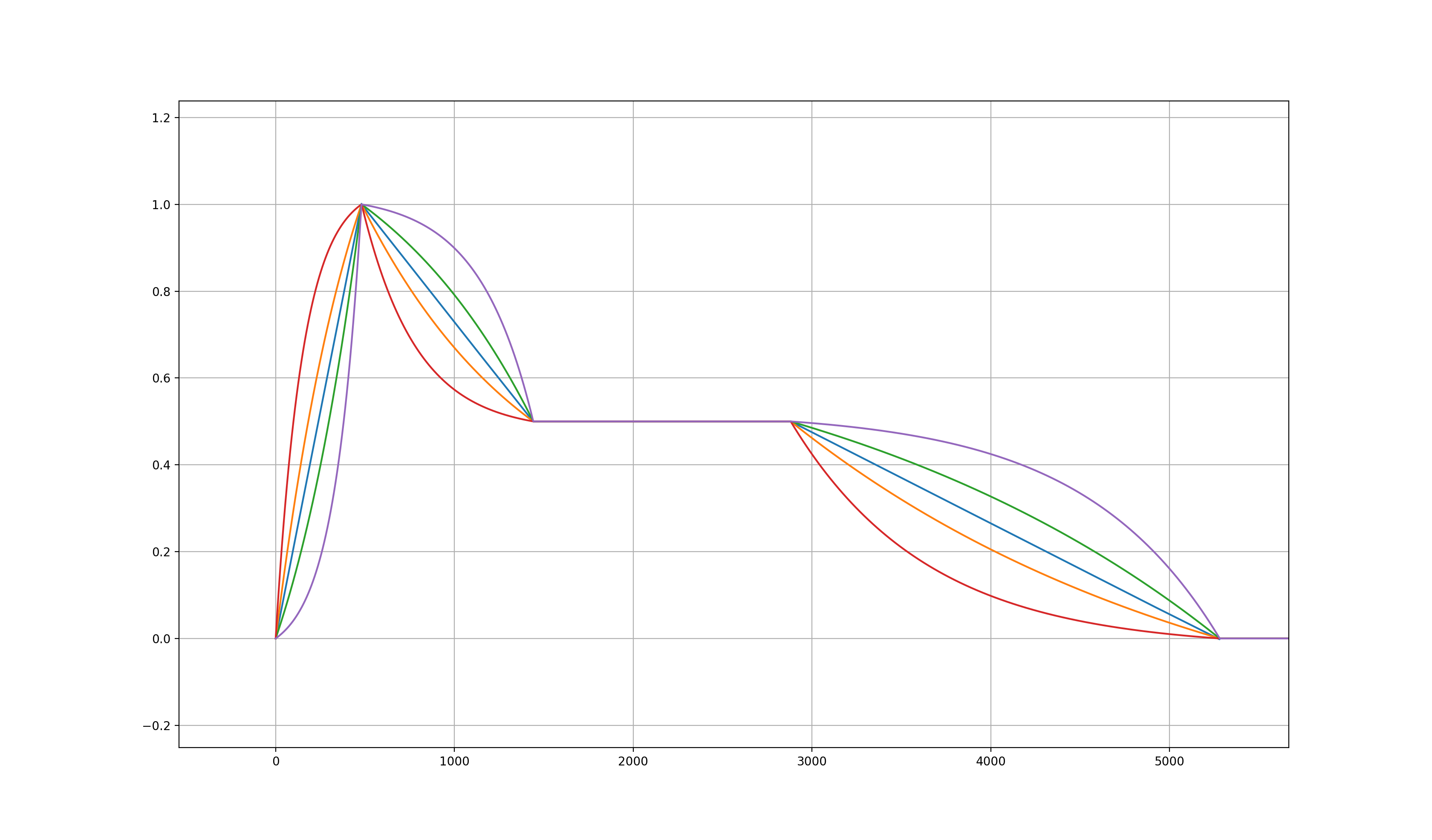
where $ x \in [0..1] $ is a real interpolation index, and $ k \neq 0 $ is a parameter determining the dis/charging rate. For values of $ k $ approaching $ 0 $, the exponential function approximates linear interpolation, whereas values further away from 0 will increase the tension of the curve in either directions. See this Desmos graph for a visual representation.
A digital one-pole filter has the form:
$$ \begin{equation} y[n] = x[n] + \alpha (y[n-1] - x[n]) \tag{2} \end{equation} $$
where the feedback coefficient is given by:
$$ \begin{equation} \alpha = e^{(-kT)/t} \tag{3} \end{equation} $$
where $ T $ is the sampling period, and $ t $ is the filter period. In other words, the step-response of the filter will reach $ 1-e^{-k} $ in the given time $ t $.
Similarly to how we normalise the output of Eq. \eqref{eq:expInter}, we can adjust the input and initial state of the filter to exponentially connect starting and ending values:
$$ y[n] = \begin{cases} y_0 & \text{if } n = 0 \\ x[n] + \alpha (y[n-1]-x[n]) & \text{if } n > 0 \tag{4} \end{cases} $$
by setting the input of the filter to the value:
$$ \begin{equation} x[n] = \frac{y_1 - y_0}{1-e^{-k}} + y_0 \quad . \tag{5} \end{equation} $$
The output of the filter closest to the target value is after $ \lfloor t / T \rceil + 1 $ samples, hence we can adjust the filter state and coefficient at the end of each segment, while the computation throughout the segment only requires one multiply and two additions. Comparing the one-pole interpolation with the exponantial mapping using std::exp() in C++, we have a mean square error equal to $ 3.777937251925323E-7 $ in single-precision processing.